Historically, neural networks have always been used as a method of deep learning, a subset of machine learning - one of the many subfields of artificial intelligence. They were first proposed about 75 years ago as an attempt at simulating the way the human brain works, though in a much more simplified form. Individual ‘neurons’ were connected in layers, with weights assigned to determine how the neuron responds when signals are propagated through the network. Previously, neural networks were limited in the number of neurons they were able to simulate, and as such, the complexity of learning they could achieve. However, in recent years, it has become possible to build very deep networks, train them on enormous datasets and hence, achieve breakthroughs in machine intelligence. These breakthroughs have allowed machines to match and exceed the capabilities of humans at performing certain tasks. One such task is image recognition. Though machines have historically been unable to match human vision, recent advances in deep learning have made it possible to build neural networks which can recognize objects, faces, text, and even emotions. In this tutorial, I will through I implemented a small subsection of object recognition—digit recognition.

Using TensorFlow, an open-source Python library developed by the Google Brain labs for deep learning, I took hand-drawn images of the numbers 0-9, built and trained a neural network to recognize and predict the correct label for the digit displayed. For anyone looking to follow these steps to build a neural network to recognize handwritten digits with TensorFlow, it is important to note that while you won’t need prior experience in practical deep learning or TensorFlow to follow along with this tutorial, some familiarity with machine learning terms and concepts such as training and testing, features and labels, optimization, and evaluation will be useful.

The building process of this project is in two parts.

• Training the deep learning model using Keras, the open-source software library that provides a Python interface for artificial neural networks whilst acting as an interface for the TensorFlow library.

• Building an interface using pygame, the cross-platform set of Python modules designed for writing video games.

Being an artificial intelligence enthusiast, this article will be focused on the former, while the latter will only be explained briefly.

The required dependencies can be found here. The .ipynb file for the deep learning model can be viewed here.

Part One

Line-by-line explanation of the Deep Learning Model.

import numpy as np
import matplotlib.pyplot as plt
import keras
from keras.datasets import mnist

This block of code imports the needed third-party dependencies.

import numpy as np imports the numpy library which can be used to perform a wide variety of mathematical operations on arrays.

import matplotlib.pyplot as plt imports the pyplot function from the matplotlib library which is used to visualize data and trends in the data.

import keras imports keras, the open-source software library that provides a Python interface for artificial neural networks whilst acting as an interface for the TensorFlow library.

from keras.datasets import mnist imports the MNIST dataset from the keras dataset library. The MNIST dataset is an acronym that stands for the Modified National Institute of Standards and Technology dataset. It is a dataset of 60,000 small square 28×28 pixel grayscale images of handwritten single digits between 0 and 9.

(X_train, y_train), (X_test, y_test) = keras.datasets.mnist.load_data()

The above line of code loads and splits the data into train set and test set.

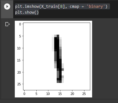
plt.imshow(X_train[8], cmap = 'binary')
plt.show()

It is important to have a view of the data. As such, I used this line of code to view the ninth element of the dataset.

The matplotlib library was used for this.

X_train = X_train.astype(np.float32)/255
X_test = X_test.astype(np.float32)/255

The block of code above normalizes the image to [0,1] range.

X_train = np.expand_dims(X_train, -1)
X_test = np.expand_dims(X_test, -1)

This block of code reshapes/expands the dimensions of images to (28,28,1)

Done cleaning the dataset, at this point, I moved on to training the model.

import tensorflow as tf
y_train = tf.keras.utils.to_categorical(y_train)
y_test = tf.keras.utils.to_categorical(y_test)

I had the block of code there in a bid to convert the class vector (integers) to binary class matrix.

from keras.models import Sequential
from keras.layers import Dense, Conv2D, MaxPool2D, Flatten, Dropout

As though I had not imported enough libraries, at this point, I imported the Sequential model. A Sequential model is usually appropriate for a plain stack of layers where each layer has exactly one input tensor and one output tensor. Furthermore, I imported five layers from the layers library. The function of each is seen thus:

1. Dense: This is just your regular densely-connected NN layer. Dense implements the operation: output = activation(dot(input, kernel) + bias) where activation is the element-wise activation function passed as the activation argument, kernel is a weights matrix created by the layer, and bias is a bias vector created by the layer (only applicable if use_bias is True).

2. Conv2D: This is the 2D convolution layer (e.g. spatial convolution over images).

3. MaxPool2D: This is used for the Max pooling operation for 2D spatial data.

4. Flatten: This flattens the input without affecting the batch size

5. Dropout: This applies Dropout to the input.

salim_model = Sequential()
salim_model.add(Conv2D(32, (3,3), input_shape = (28,28,1), activation = 'relu'))
salim_model.add(MaxPool2D(2,2))


salim_model.add(Conv2D(64, (3,3), activation = 'relu'))
salim_model.add(MaxPool2D(2,2))

salim_model.add(Flatten())

salim_model.add(Dropout(0.25))

salim_model.add(Dense(10, activation = 'softmax'))

After initializing the model under the variable name salim_model, i then used the previously imported layers with suitable parameters.

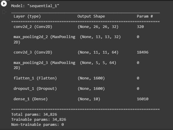
salim_model.summary()

In a bid to ascertain that the model was well-trained to my taste, I used the .summary() function to take a peek.

salim_model.compile(optimizer = 'adam', loss = keras.losses.categorical_crossentropy, metrics = ['accuracy'])

I then configured the model for training using adam as the optimizer. See more optimizers here. Furthermore, I choose to use accuracy as the metric for evaluating my model.

his = salim_model.fit(X_train, y_train, epochs = 5, validation_split = 0.25, callbacks = cb)

I then finally train my model with 25% of the dataset dedicated to validation in five epochs.

After the fifth epoch, an accuracy of 99.85% was seen.

salim_model.save('my_model.h5')

Finally, I saved the model to be used in the pygame script under the name, my_model.h5.

Part Two

Delivering the model

Now, Deep Learning is cool but what I consider even cooler is Deep Learning in production. So whilst I already has a model that recognizes human-written to an accuracy of about 98%, I needed to deploy it for use. Although a number of methods came up, I opted to harness the pygame module. Using the model, I was able to create a window that recognizes the written number and accurately predict the number.

However, I still had a problem. This model could only be tested locally. I needed to make it shareable. As such, I used the cx_Freezer to convert the model into an executable file (EXE file).

The link to the full code can be found here