Linear regression is a type of supervised learning algorithm where the output is in a continuous range and isn’t classified into categories. Through a linear regression machine learning algorithm, we can predict values with a constant slope. Just as the Naive Bayes Algorithm is a good starting point for classification tasks, Linear Regression models are a good starting point for regression tasks. Such models are popular because they can be fit very quickly, and are very interpretable. If you are not new to the data science/machine learning space, you are probably familiar with the simplest form of a linear regression model (i.e., fitting a straight line to data), but such models can be extended to models more complicated. In this article, I will give a quick walk-through of the mathematics behind this well-known model.

Regression as a broad concept is a common process used in many applications of statistics in the real world. There are two main types of its applications:

Predictions: After a series of observations of variables, regression analysis gives a statistical model for the relationship between the variables. This model can be used to generate predictions: given two variables x and y, the model can predict values of y given future observations of x. This idea is used to predict variables in countless situations, e.g. the outcome of political elections, the behavior of the stock market, or the performance of a professional athlete.

Correlation: The model given by a regression analysis will often fit some kinds of data better than others. This can be used to analyze correlations between variables and to refine a statistical model to incorporate further inputs: if the model describes certain subsets of the data points very well, but is a poor predictor for other data points, it can be instructive to examine the differences between the different types of data points for a possible explanation. This type of application is common in scientific tests, e.g. of the effects of a proposed drug on the patients in a controlled study.

Consider the following data, which is scattered about a line with a slope of 3 and an intercept of –4

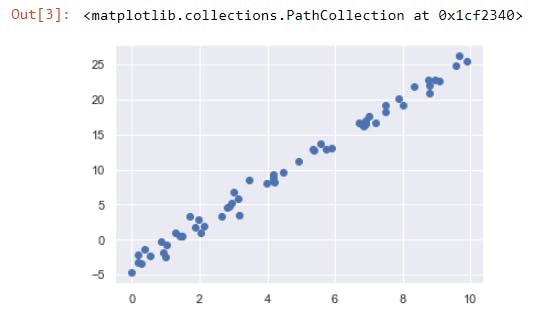
Data for linear regression

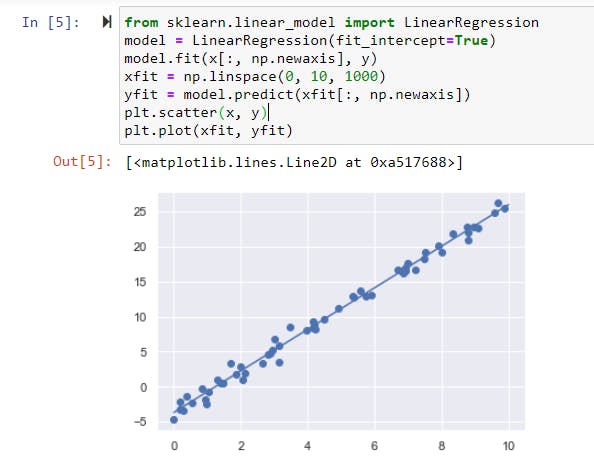
We can use Scikit-Learn’s LinearRegression estimator to fit this data and construct the best-fit line.

from sklearn.linear_model import LinearRegression
model = LinearRegression(fit_intercept=True)
model.fit(x[:, np.newaxis], y)
xfit = np.linspace(0, 10, 1000)
yfit = model.predict(xfit[:, np.newaxis])
plt.scatter(x, y)
plt.plot(xfit, yfit)

And then, we have;

In the simplest form, here is what the ML model looks like.

As shown above graphically, the task is to draw the line that is "best-fitting" or "closest" to the points (xi, yi), where xi and yi are observations of the two variables which are expected to depend linearly on each other. This can only be achieved by the principle of ordinary least square (OLS) / Mean square error (MSE). That is, viewing y as a linear function of x, the method finds the linear function L which minimizes the sum of the squares of the errors in the approximations of the yi by L(xi).

To show this method, another dataset will be used;

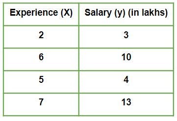Given is a Work vs Experience dataset of a company and the task is to predict the salary of a employee based on his / her work experience.

The aim is to explain how in reality Linear regression mathematically works when we use a pre-defined function to perform prediction task.

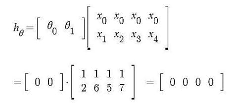
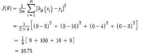
Iteration 1 – In the start, θ0 and θ1 values are randomly chosen. Let us suppose, θ0 = 0 and θ1 = 0. Predicted values after iteration 1 with Linear regression hypothesis.

Cost Function – Error

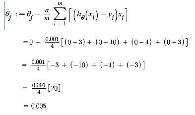
Gradient Descent – Updating θ0 value Here, j = 0

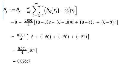
Gradient Descent – Updating θ1 value Here, j = 1

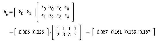
Iteration 2 – θ0 = 0.005 and θ1 = 0.02657 Predicted values after iteration 1 with Linear regression hypothesis.

Now, similar to iteration no. 1 performed above we will again calculate Cost function and update θj values using Gradient Descent. We will keep on iterating until Cost function doesn’t reduce further. At that point, model achieves best θ values. Using these θ values in the model hypothesis will give the best prediction results.