Project 3 - House Prices Prediction using Machine Learning with Python

I am Salim Olanrewaju Oyinlola. I identify as a Machine Learning and Artificial Intelligence enthusiast who is quite fond of making use of data and patterns to develop insights and analysis.

In my opinion, Machine learning is where the computational and algorithmic skills of data science meets the statistical thinking of data science. The result is a collection of approaches that requires effective theory as much as effective computation. There are a plethora of machine learning model, with each of them working best for different problems. As such, I believe understanding the problem setting in machine learning is essential to using these tools effectively. Now, the best way to UNDERSTAND different problem settings is by PLAYING AROUND with different problem settings. That is the genesis behind this writing series - My Machine Learning Projects. Over the course of this writing series, I would solve a machine learning problem daily. These problems will range from a plethora of fields whilst requiring and covering a range of models. A link to my previous articles can be found here.

Project Description: This is a regression problem that uses the boston house prices dataset collected by Harrison, D. and Rubinfeld, D.L. in determining/predicting the prices of houses in the Boston suburb area.

URL to Dataset: SKLearn's pre-loaded data collected from houses in Boston’s suburbs collected by Harrison, D. and Rubinfeld, D.L.

Line-by-line explanation of Code

import numpy as np
import pandas as pd
import matplotlib.pyplot as plt
import seaborn as sns
import sklearn.datasets
from sklearn.model_selection import train_test_split
from xgboost import XGBRegressor
from sklearn import metrics

The block of codes above imports the third party libraries used in the model.

import numpy as np imports the numpy library which can be used to perform a wide variety of mathematical operations on arrays.

import pandas as pd imports the panda library which is used to analyze data.

import matplotlib.pyplot as plt imports the pyplot function from the matplotlib library which is used to visualize data and trends in the data.

import seaborn as sns imports the seaborn library which is used for making statistical graphics. It builds on top of matplotlib and integrates closely with pandas data structures. Seaborn helps you explore and understand your data.

import sklearn.datasets imports library containing sklearn's datasets that comes pre-installed with sklearn.

from sklearn.model_selection import train_test_split imports the train_test_split function from sklearn's model_selection library. It will be used in spliting arrays or matrices into random train and test subsets.

from xgboost import XGBRegressor imports the XGBoost Machine Learning model from xgboost third party library. XGBoost stands for Extreme Gradient Boosting and it is an implementation of gradient boosting trees algorithm. The XGBoost is a popular supervised machine learning model with characteristics like computation speed, parallelization, and performance.

Note: xgboost is a third-party module in python and as such, must be pip installed before use.

from sklearn import metrics imports the metric library used to ascertain the performance of our model.

salim_house_price_dataset = sklearn.datasets.load_boston()

This line of code loads/reads the dataset and saves it in the variable salim_house_price_dataset.

salim_house_price_dataframe = pd.DataFrame(salim_house_price_dataset.data, columns = salim_house_price_dataset.feature_names)

This line of code loads the dataset to a Pandas DataFrame.

salim_house_price_dataframe.head()

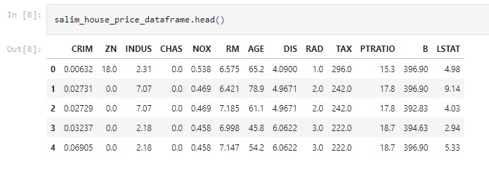
This line of code prints the first 5 rows of the DataFrame.

Thirteen (13) attributes are seen as follows;

1. CRIM - Capita crime rate by town
2. ZN - proportion of residential land zoned for lots over 25,000 sq. ft.
3. INDUS - proportion of non-rental business acre per town.
4. CHAS - Charles River dummy variable {= 1 if tract bounds river, 0 otherwise}
5. NOX - Nitric Oxide concentration {parts per 10 million}
6. RM - Average number of rooms per dwelling.
7. AGE - Proportion of owner-occupied on its built prior to 1940
8. DIS Weighted distances to five Boston employment centres
9. RAD - Index of accessibility to radial highways
10. TAX -Full-value property-tax rate per $10,0000
11. PTRATIO - Pupil-Teacher ratio by town
12. B - 1000(BK-0.63)^2 where BK is proportion of blacks by town.
13. LSTAT - Lower status of the population

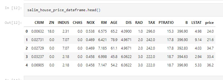
salim_house_price_dataframe['price'] = salim_house_price_dataset.target

This line of code adds the target (price) column to the DataFrame.

salim_house_price_dataframe.head()

This prints the first 5 rows of the DataFrame with the target (price)

salim_house_price_dataframe.shape

This line of code is used for checking the number of rows and Columns in the data frame

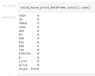
salim_house_price_dataframe.isnull().sum()

This line of code checks for missing values. We see that there is no missing value.

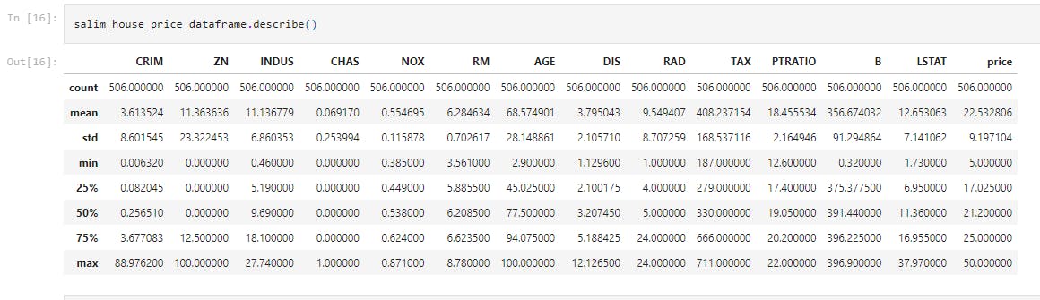
salim_house_price_dataframe.describe()

This displays the statistical measure of the data (i.e. the mean, median, max, min 25th, 50th and 75th percentile values.)

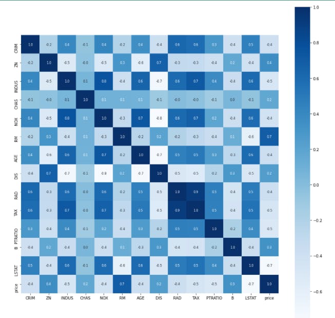
correlation = salim_house_price_dataframe.corr()
plt.figure(figsize=(15,15))
sns.heatmap(correlation, cbar=True, square=True, fmt='.1f', annot=True, annot_kws={'size':8}, cmap='Blues')

This block of code constructs a heatmap to understand the correlation.

X = house_price_dataframe.drop(['price'], axis=1)
Y = house_price_dataframe['price']

This separates data and Labels.

X_train, X_test, Y_train, Y_test = train_test_split(X, Y, test_size = 0.2, random_state = 4)

The train_test_split method that was used earlier is hence called and used to divide the dataset into train set and test set.

• The 0.2 value of test_size implies that 20% of the dataset is kept for testing whilst 80% is used to train the model.

model = XGBRegressor()

This loads the model by creating an instance of the XGB Regressor Machine Learning Algorithm.

model.fit(X_train, Y_train)

This trains the model with X_train.

salim_training_data_prediction = model.predict(X_train)

This evaluates the accuracy for prediction on training data.

score_1 = metrics.r2_score(Y_train, salim_training_data_prediction)

score_2 = metrics.mean_absolute_error(Y_train, salim_training_data_prediction)

print("R squared error : ", score_1)
print('Mean Absolute Error : ', score_2)

score_1 is the # R squared error

score_2 is the # Mean Absolute Error

In my model, we see a 0.9999911407789398 R Squared error and 0.01893801547513154 as the mean absolute error.

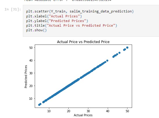
plt.scatter(Y_train, salim_training_data_prediction)
plt.xlabel("Actual Prices")
plt.ylabel("Predicted Prices")
plt.title("Actual Price vs Predicted Price")
plt.show()

For better visualization, I plotted a graph of the Actual Prices against Predicted Prices. A linear graph is observed.

salim_test_data_prediction = model.predict(X_test)

score_1 = metrics.r2_score(Y_test, salim_test_data_prediction)


score_2 = metrics.mean_absolute_error(Y_test, salim_test_data_prediction)

print("R squared error : ", score_1)
print('Mean Absolute Error : ', score_2)

This line of code determines the accuracy for prediction on test data.

score_1 is the # R squared error

score_2 is the # Mean Absolute Error

In my model, we see a 0.8305367046415144 R Squared error and 2.417451073141659 as the mean absolute error.

That's it for this project. Be sure to like, share and keep the discussion going in the comment section. .ipynb file containing the full code can be found here.