I am Salim Olanrewaju Oyinlola. I identify as a Machine Learning and Artificial Intelligence enthusiast who is quite fond of making use of data and patterns to develop insights and analysis.

In my opinion, Machine learning is where the computational and algorithmic skills of data science meets the statistical thinking of data science. The result is a collection of approaches that requires effective theory as much as effective computation. There are a plethora of machine learning model, with each of them working best for different problems. As such, I believe understanding the problem setting in machine learning is essential to using these tools effectively. Now, the best way to UNDERSTAND different problem settings is by PLAYING AROUND with different problem settings. That is the genesis behind this writing series - My Machine Learning Projects. Over the course of this writing series, I would solve a machine learning problem daily. These problems will range from a plethora of fields whilst requiring and covering a range of models. A link to my previous articles can be found here.

Project Description: This project is a classification model to determine if loan applications are eligible.

URL to Dataset: Download here

Line-by-line explanation of Code

import numpy as np
import pandas as pd
import seaborn as sns
from sklearn.model_selection import train_test_split
from sklearn import svm
from sklearn.metrics import accuracy_score

The block of codes above imports the dependencies used in the model.

import numpy as np imports the numpy library which can be used to perform a wide variety of mathematical operations on arrays.

import pandas as pd imports the panda library which is used to analyze data.

import seaborn as sns imports the seaborn library which is used for making statistical graphics. It builds on top of matplotlib and integrates closely with pandas data structures. Seaborn helps you explore and understand your data.

from sklearn.model_selection import train_test_split imports the train_test_split function from sklearn's model_selection library. It will be used in spliting arrays or matrices into random train and test subsets.

from sklearn import svm imports the Support Vector Machine (SVM) Machine Learning model from the sklearn library. This model will be used in training the model.

from sklearn.metrics import accuracy_score imports the accuracy_score function from sklearn's metrics library. This model is used to ascertain the performance of our model.

• The Support Vector Machine(SVM) is a supervised machine learning algorithm used for both classification and regression. Though we say regression problems as well its best suited for classification.

salim_loan_dataset = pd.read_csv(r'C:\Users\OYINLOLA SALIM O\Downloads\fake-news/train_u6lujuX_CVtuZ9i (1).csv')

This line of code reads the dataset.

type(salim_loan_dataset)

This line of code returns the type of the values in the dataset. On running, pandas.core.frame.DataFrame is returned.

salim_loan_dataset.head()

This line of code prints the first 5 rows of the dataframe.

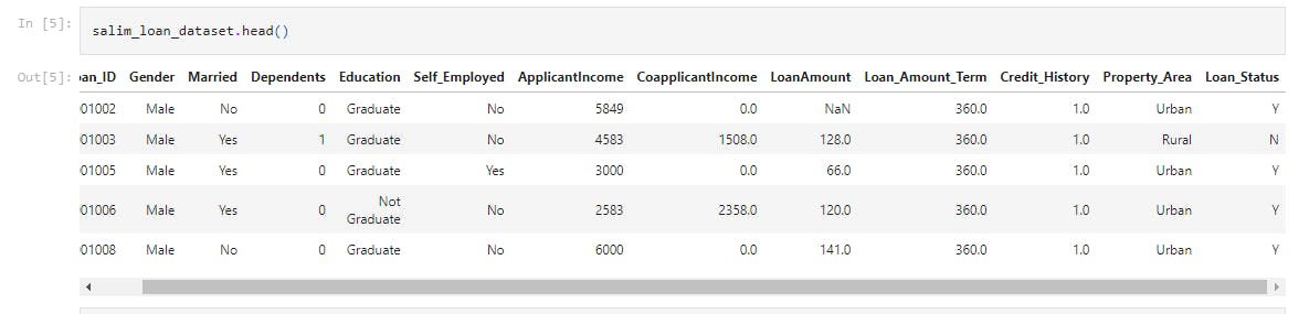
The following attributes are seen;

Gender, Married, Dependents, Education, Self_Employed, ApplicantIncome, CoapplicantIncome, LoanAmount, Loan_Amount_Term, Credit_History, Property_Area, Loan_Status;

salim_loan_dataset.shape

This returns the number of rows and columns. We see (614, 13)

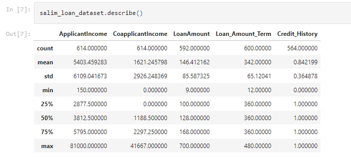
salim_loan_dataset.describe()

This displays the statistical measure of the data (i.e. the mean, median, max, min 25th, 50th, 75th percentile values etc.)

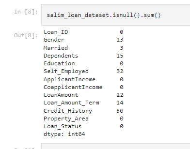
salim_loan_dataset.isnull().sum()

This returns the number of null values in the data.

salim_loan_dataset = loan_dataset.dropna()

This drops the missing values.

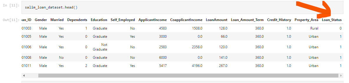
salim_loan_dataset['Loan_Status'] = salim_loan_dataset['Loan_Status'].map({'Y':1 ,'N':0})

This process is called label encoding. It converts the string values of Y and N in the Loan_Status column to 1 and 0 respectively.

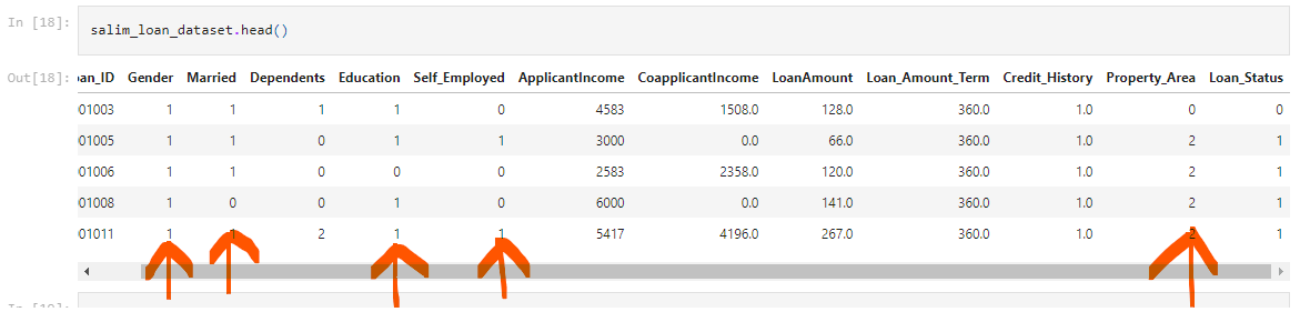
salim_loan_dataset.head()

This was used to see the first five rows again to be sure the label encoding process took full effect.

salim_loan_dataset['Dependents'].value_counts()

This returns the respective entries in the Dependents column with the frequency of occurence as seen. 0 274 2 85 1 80 3+ 41

salim_loan_dataset = salim_loan_dataset.replace(to_replace='3+', value=4)

This replaces the value of 3+ to 4.

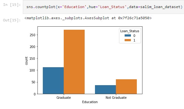
sns.countplot(x='Education',hue='Loan_Status',data=salim_loan_dataset)

This line of code uses the seaborn library to draw a countplot of the Education status of loan applicants.

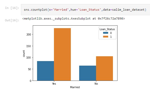
sns.countplot(x='Married',hue='Loan_Status',data=salim_loan_dataset)

This line of code uses the seaborn library to draw a countplot of the Married column for the dataset.

salim_loan_dataset.replace({'Married':{'No':0,'Yes':1},'Gender':{'Male':1,'Female':0},'Self_Employed':{'No':0,'Yes':1},
                      'Property_Area':{'Rural':0,'Semiurban':1,'Urban':2},'Education':{'Graduate':1,'Not Graduate':0}},inplace=True)

This process is called label encoding. It replaces texts with numerical values. In the Married column, No is replaced with 0 and Yes is replaced with 1.

In the Gender column, Male is replaced with 1 and Female is replaced with 0

In the Self_Employed column, Yes is replaced with 1 and No is replaced with 0

In the Property_Area column, Rural is replaced with 0, Semiurban is replaced with 1 and Urban is replaced with 2

In the Education column, Graduate is replaced with 1 and Not Graduate is replaced with 0

salim_loan_dataset.head()

This line of code prints the first 5 rows of the dataset to ascertain that the changes have been made.

X = salim_loan_dataset.drop(columns=['Loan_ID','Loan_Status'],axis=1)
Y = salim_loan_dataset['Loan_Status']

This block of code separates the data & label.

X_train, X_test,Y_train,Y_test = train_test_split(X,Y,test_size=0.1,stratify=Y,random_state=2)

The train_test_split method that was used earlier is hence called and used to divide the dataset into train set and test set.

• The 0.2 value of test_size implies that 20% of the dataset is kept for testing whilst 80% is used to train the model.

classifier = svm.SVC(kernel='linear')

Initializing an instance of the Support Vector Classifier part of the Support Vector Machine (Since SV, encpmapsses classification and regression)

print(X.shape, X_train.shape, X_test.shape)

This returns the number of X values, the number of those values that are in the train set and the number of them in the test set.

classifier.fit(X_train,Y_train)

This trains the support vector Machine Classifier with the train dataset.

X_train_prediction = classifier.predict(X_train)
training_data_accuray = accuracy_score(X_train_prediction,Y_train)
print('Accuracy on training data : ', training_data_accuray)

This block of code evaluates the accuracy score on the training data. We see an accuracy score of 0.7986111111111112.

X_test_prediction = classifier.predict(X_test)
test_data_accuray = accuracy_score(X_test_prediction,Y_test)
print('Accuracy on test data : ', test_data_accuray)

This block of code evaluates the accuracy score on the test data. We see an accuracy score of 0.8333333333333334.

That's it for this project. Be sure to like, share and keep the discussion going in the comment section. .ipynb file containing the full code can be found here.